Hey!

Conway’s Game of Life is one of the coolest interactive examples of the beauty of mathematics. But realize that it’s only interactive because a huge community of people have chosen to interact with it – to build tools to toggle cells in a grid while operation is paused, then unpause and see what happens to our creations. There’s an encyclopedia of oscillators, gliders, transistors, memory circuits, self-replicating spaceships, and even modular computers that simulate the Game of Life within itself, all written in a language of cells that live or die according to one extremely simple function of how many of their nearest neighbors are living. Constructs in Conway’s Game of Life are written in a language that transcends our cultures and the physical context of our universe. If we etched a Gosper Glider Gun into a golden record on some future space probe, there’s a decent chance that any alien civilization to recover that record would recognize it as something they’ve already discovered and named, like the Mandelbrot set.

Anyway, trying to read through that encyclopedia of community knowledge made it very clear to me that looking to other rules for cellular automata was not necessary for the pure purpose of finding fresh challenges – the frontier of discovery within the Game of Life is plenty big and plenty accessible, and half a century after its conception, things are only ramping up with more sophisticated programs for accelerating the simulation and searching for patterns.

But I took the option of wondering what else there is, and what even Golly (the most famous and advanced cellular automata tool) doesn’t show me. There’s a reason why cellular automata with float states probably aren’t as much fun to play with – too much chaos with no way to bring it under control. Conway’s Game of Life is often chaotic, but at least with quantization of both cell positions and cell states, everything falls into some assortment of smaller patterns that we can visually identify, give names to, and make generalizations about. Draw any random shape of a dozen live cells in the Game of Life and watch it decompose into moving “gliders” and stationary “stoplights” and “beehives” and other things – none of them will interfere with or destroy another except by the general rules that can describe each of them in a vacuum. Two gliders either collide with each other, or pass by each other with no interaction of any kind. In a world without integer states for cells, I strongly suspect that it is difficult for any machine that can exist in a vacuum to co-exist with a nearby copy of itself or another machine – it might be like trying to fly an airplane in a world with other airplanes, but the wake turbulence travels in all directions at the speed of light, and instead of the turbulence being made of air, it’s made of a torrent of solid airplane parts.

This is a problem affecting most 2-dimensional cellular automata rules. The good rules must be sought out, and Life is one of them. It doesn’t make sense to ask whether Life is self-regulating, and the answer might seem to be no (since one misplaced cell can destroy a creation of any size), but it doesn’t seem to matter because of how any finite area in Life has a finite number of states. The state of an area is the same as the code that controls what it will do, and this is why a glider will glide no matter what goes on around it, as long as those events don’t change the cells inside the bounding area of the glider. In a world with infinite states for any area of any size, two gliders passing each other might destroy each other by default, because infinitesimal effects on each other might push them out of whatever distinct shape of ranges of cell states act glider-like.

Nevertheless, I decided that cellular automata with non-integer states were well worth experimenting with – maybe only because they pack infinitely more information into the same number of calculations, and because I didn’t know what there was to learn – are they good for computing? Is there a rule that’s good for building computing machines out of cells – maybe even more compactly than in Conway’s Game of Life?

Or,

Is there a rule in the form Z -> sin(sum(neighbors of Z)*a)^b which behaves similarly to Conway’s Game of Life? (A rule where large machines can be built from smaller machines, where oscillators and spaceships can exist, and where the appearance of complete chaos is avoided?)

My latest project FloatAutomata.py aims to discover this.

github.com/JohnDorsey/FloatAutomata.git

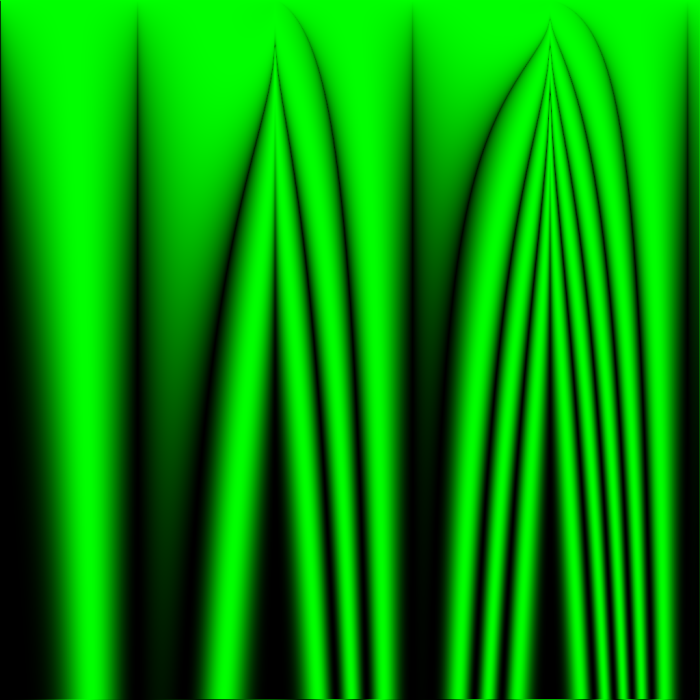
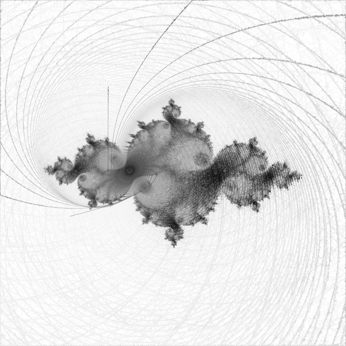
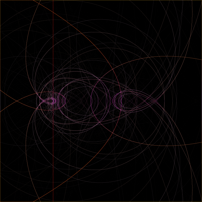
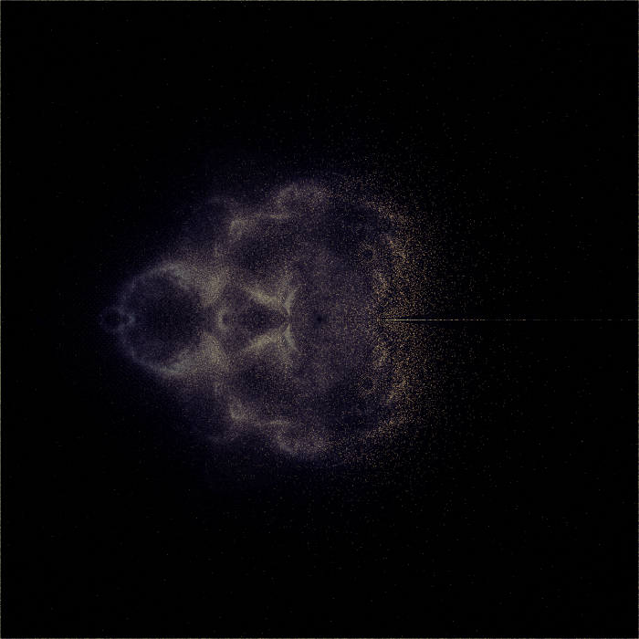
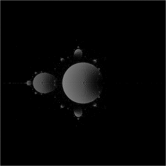
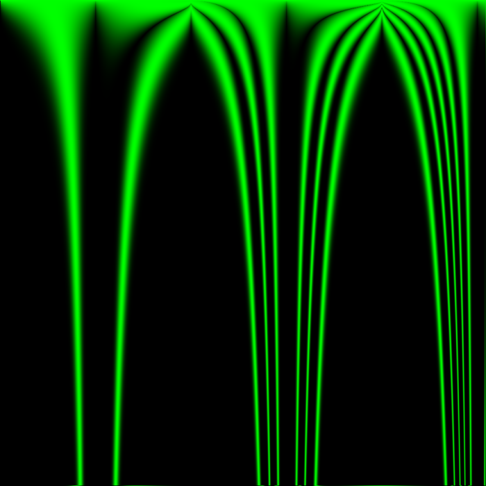
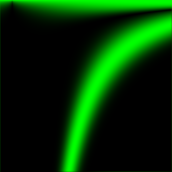
In my recent simulations, I aim to search for ideal rules by testing all rules at once in a shared grid. Each cell’s position determines the parameters of the rule to be used, seen as the variables x and y in the image caption. Although no cell can interact with cells of the same rule, each cell will be interacting with cells of highly similar behavior, hopefully leading to large areas of an image all demonstrating good orderly behavior in areas centered around the pixel with the perfect parameters to create that behavior – just as the Mandelbrot set mimics whatever Julia set is formed by the value C equal to that location, but never perfectly re-creates a Julia set.

Y is measured from the top of the image in pixels, so in these 1024×1024 images, a rule definition which contains (y/512) means that that expression will range from 0 to 2 between the top edge of the image and the bottom edge.

In this entire post, I never resample images – each pixels corresponds to exactly one cell. Every cell state between 0.0 and 1.0 maps to a green channel value between 0 and 255 unless otherwise stated. Every simulation starts with all cells set to 0.5 unless otherwise stated.

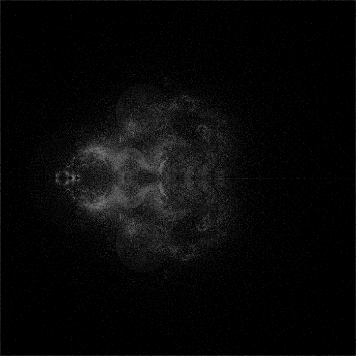
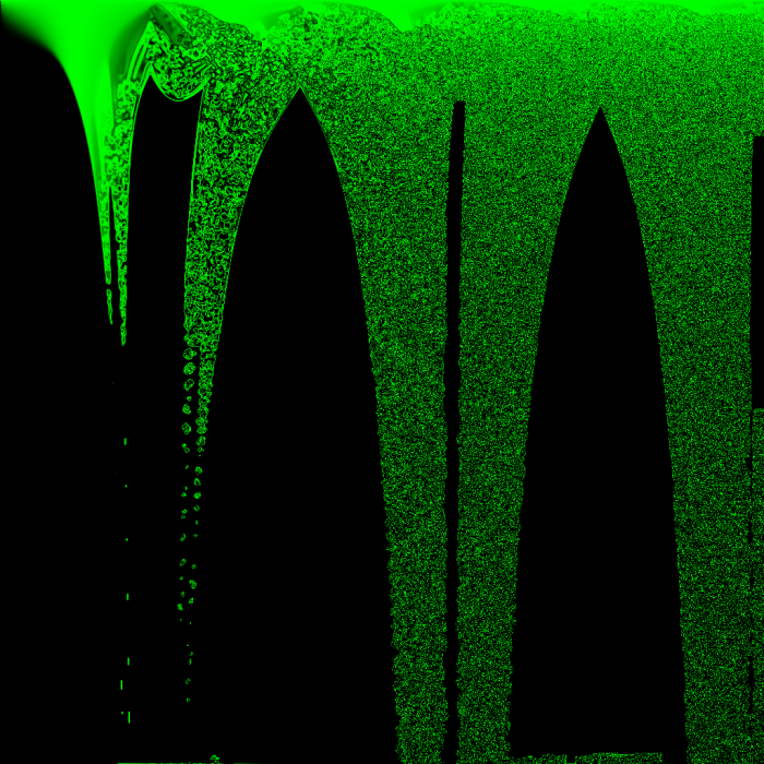
The above image of the world at 64 iterations shows that, at least with the way I am choosing to initialize the world, there are no groups of similar rules that all create sparse activity. From images like these, I can’t determine what a only a few live cells would do in a vacuum, because none of them are alone without constant outside interference from other nearly-random cells… Starting with a few live cells is one of the best ways to demonstrate the strengths of Conway’s rule for creating complex organized motion, and this simulation doesn’t do that.

Good rules might be in there, and they just aren’t being given a fair chance at demonstrating order.

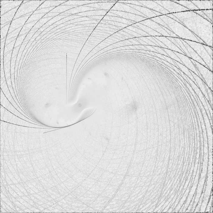
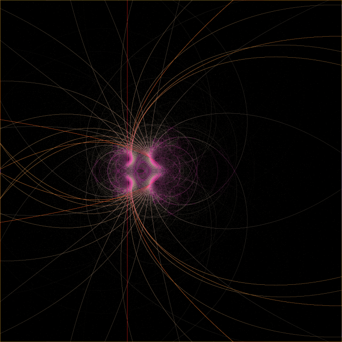
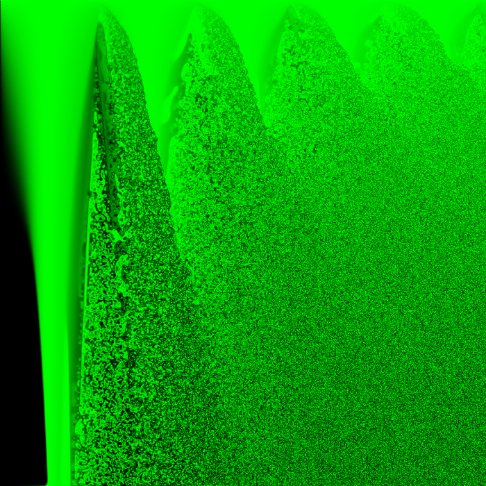
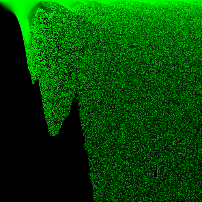
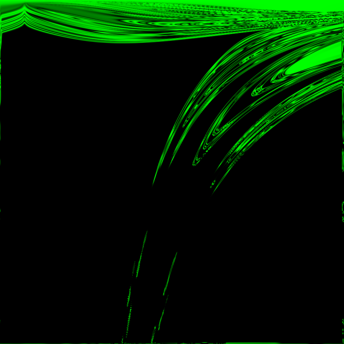
This render is simply the first render zoomed out. Since there’s one cell per pixel, zooming out changes the number of cells in any area within the space of the parameters used for the rule, so zooming out must change the observed behavior of every part of the world. Cells that previously had neighbors with rule parameters different from their own by 1/512 now have neighbors with rule parameters different from their own by 1/64.

I zoomed out this far because I didn’t want to miss an interesting rule, but what I learned from zooming out this far was discouraging…

The noise bleeds like ink until it fills up the whole world.

Generally, in Conway’s Game of Life, endless growth (of live cell population) is something that needs to be designed, not something that happens randomly. I can think of only one situation in which Conway’s Game of Life produces unlimited chaos…

In an experiment I did in Golly, I required an infinite world of repeating gliders, and I used the preset pi-blink-breeder2 under patterns>Life>breeders.

The pattern info includes this attribution:

#C An unusual breeder (quadratic growth) pattern.
#C By Jason Summers and David Bell, 6 Sep 2002; from "jslife" archive.

The breeder (a machine that constructs machines that construct gliders) is not important to the experiment – I am only concerned with the area of gliders it produces. In their midst, I drew exactly one glider traveling in the opposite direction, so that it collided with one of them after a while, and this was the result:

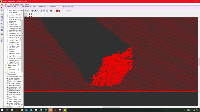
That’s essentially a ~200,000-car pileup, which would continue to grow infinitely if it didn’t hit the breeder’s wick of glider builders. In the best-behaved rule that I know of, all it takes to get an infinite chaotic mess is for the world to be initially full (of gliders).

If all I could see of this simulation were a section of the chaos coral, and I were asked whether I thought the rule that created it were Turing-complete, I might say “not really, I mean, you couldn’t practically make a computer out of it like you can with Life” not knowing that I was looking at Life.

I’m saying that none of my experiments so far offer strong evidence that a life-like rule using a sine function either does or doesn’t exist. In future experiments, I should test sine-based rules the same way I test rules by hand in Golly – apply the same rule to the whole world, edit in a handful neighboring live cells in a small random shape that isn’t symmetrical, and hit the play button. In FloatAutomata.py, this would look like quantizing the parameters of rules to make areas of about 64×64 cells that all have exactly the same rule, and not starting the simulation with every cell equal to 0.5. Each square of one rule should start with only a handful of nonzero cells in a cluster near the center.

In the meantime, here are the other experiments I’ve already performed with the whole world starting as 0.5-filled:

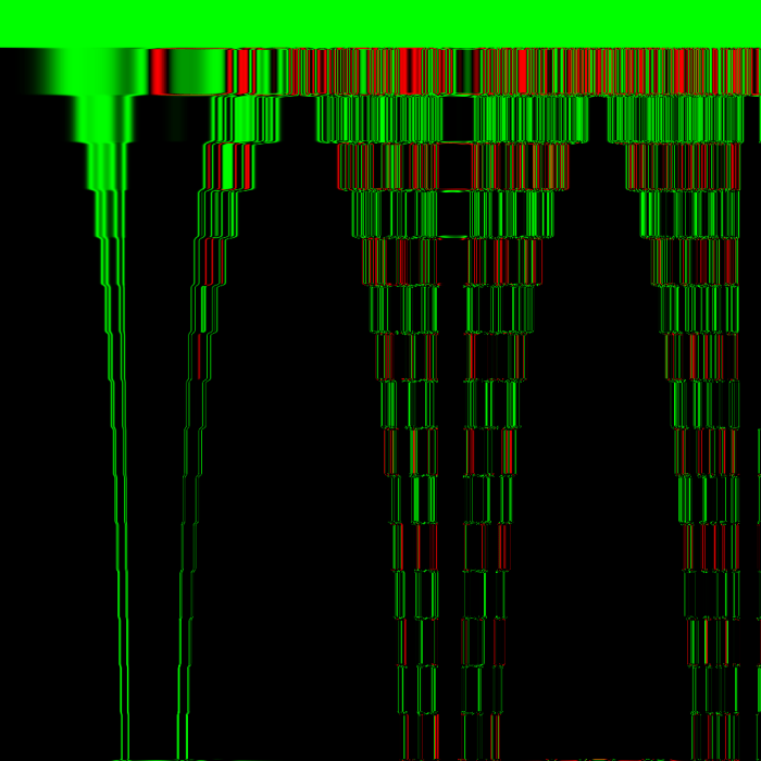
It might seem like the boundary areas between emptiness and noise are good candidates for well-behaved rules, but I think that if this were true, the boundary areas would not constantly be moving!

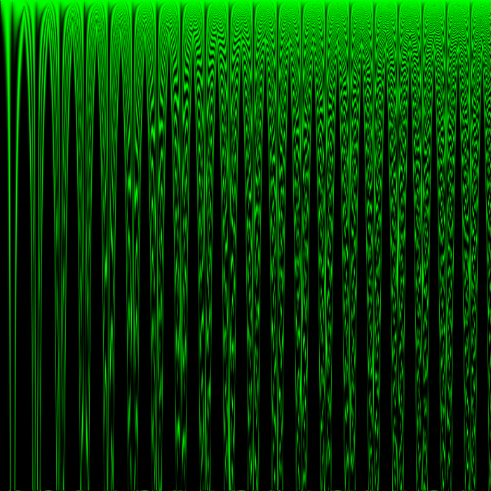
Also note that toroidal wrap was enabled for every one of these experiments, and its effects can sometimes be seen in noise leaking in from the edges of an image to a maximum distance in pixels equal to the number of iterations to happen so far – it’s just because they were exposed to pixels on the opposite edge of the image. It usually doesn’t impact the image at the top or left edges, where one of the parameters is usually zeroed out anyway. For example, in the above image of Z -> abs(sin(sum(neighbors)*x/512))^(y/64) after 16 iterations, the bottom edge of the image has a line of noise caused by exposure to the top edge, but the top edge has no such line of noise.

In the above images, anything that looks noisy is located very close to an area that was active in previous iterations – there are no gliders, and all things that look like islands of stability seem to eventually die. Except for two! their coordinates are (429, 720) and (518, 762), giving them the approximate rules:

Z -> abs(sin(sum(neighbors)*0.479736328125))^(11.25)
Z -> abs(sin(sum(neighbors)*0.50146484375))^(11.90625)

These will be investigated at a later date.

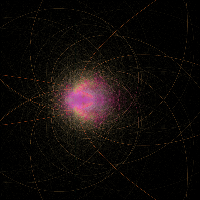
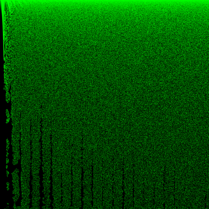
Even so, the above images serve to demonstrate that which areas of the image appear vital and stable is highly dependent on which areas of the image had ideal starting conditions from the few iterations after the world’s creation, which in turn depends on which rules are good at creating chaos from a starting neighborhood of 8 cells all with the state 0.5.

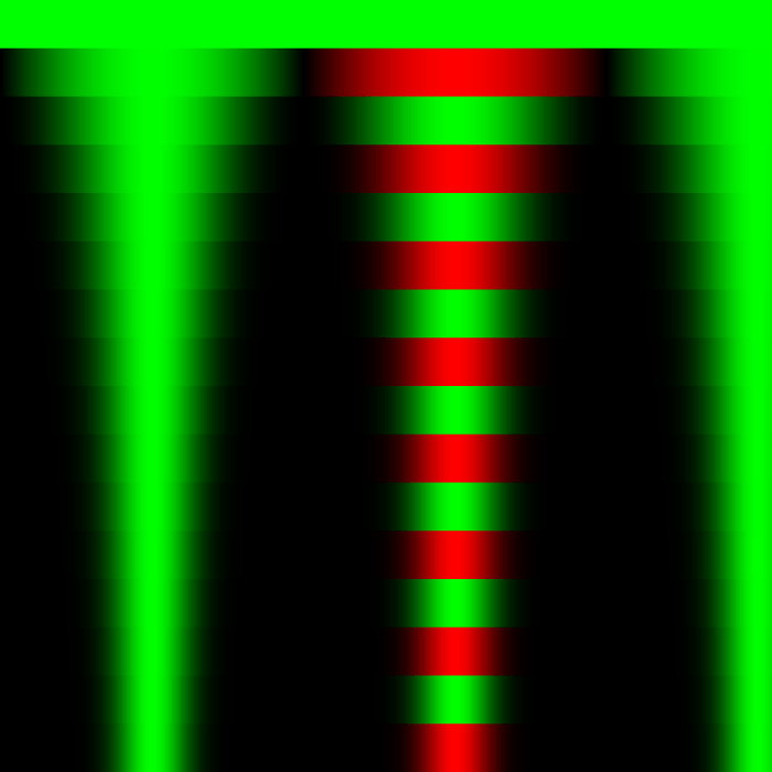
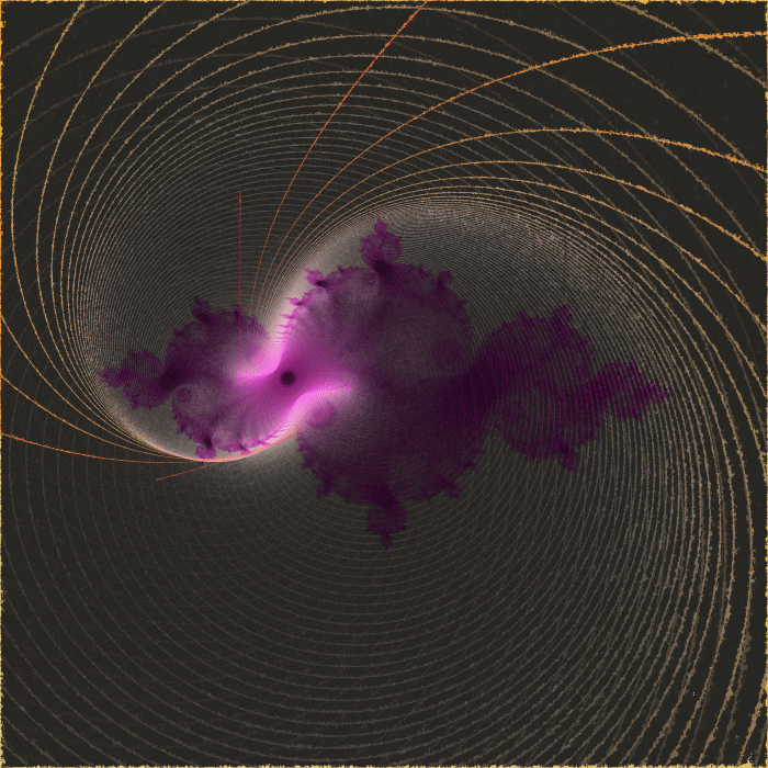
A new color palette has been introduced – reds code for negative values in the same range as greens. Negative numbers are allowed now that exponents are limited to integers – I didn’t want to deal with complex math on my first day of experimenting.

Note in the center left of the image, near the bottom end of the second of the image’s four tornado shapes, there appears to be a symmetrical barcode shape – animated over time, this looks like traveling along a binary tree layer by layer. Conway’s Game of Life never does this, but I believe some other cellular automata with binary states do. Just like what is seen here, those rules produce growing regions of noise at either end of a barcode’s bars until the barcode is consumed by the noise. In this experiment, the barcodes are initially stretched between the boundary lines of integer exponents in the rule (64 pixels per integer value).

I may upload additional experiments of the same type before continuing to testing of individual rules with more fair (non-solid) starting states of the world. I will also cover some surprisingly orderly rules using the tangent function!

The entire project is available on GitHub to view and download. It requires only Python to run. If you also have Pygame installed, it is used to draw graphs that supplement the console output.

---

For my semester project in 2017, I decided to finalize a program I had already been working on for several months as a hobby: An algorithm to travel between any two input numbers, using only the operations from the Collatz Conjecture to construct a path.

My goals for this project:

• Demonstrate that a transformation between any two positive integers can be created by applying 4 unique operations in a finite sequence,
• Compute the shortest sequence for two input numbers,
• Provide an example of how these sequences can be used in cryptography.

In the Collatz conjecture, the appropriate operation is chosen based on whether N is even or odd; N->N/2 is applied only when N is even, N->3N+1 is used otherwise. This ensures that N remains an integer, but also allows only one sequence of operations to occur after the starting point N. In my program, the inverses of these two operations (N->2N, N->(N-1)/3) are also available, and an operation is allowed whenever the result is an integer.

This gives freedom of movement throughout the number line.

Rather than selecting new operations based on a rule regarding the current number, a sequence can be created by an outside program, which has memory (See: the difference between Langton’s Ant and Langton himself). The numbers visited are like intersections in a maze, and the sequence generator acts like a maze solver.

I did not know about graph theory when I created this, but I ended up creating a breadth-first undirected graph search. The graph consists of all numbers which satisfy the Collatz conjecture, and the edges are the 4 operations.

The first version of the program was not so advanced – it searched by iteratively choosing the option which was closest to the target number, but avoiding numbers which had already been used. This was inefficient, and not set up to find the shortest path.

The quickest path to the target number would never be guessed by this solver, if any of the steps in the quickest path were not the longest steps that could be taken. That is to say, when creating a path from 64 to 256:
64 (*2) -> 128 (*2) -> 256
would always be turned down in favor of:
64 (*3+1) -> 193 -> (a lot of aimless wandering) -> 256

Originally, the stacked solver could become barred from reaching the goal by a wall of numbers that it had already used, and would be forced to walk further and further from the goal until it ran out of memory. (Even with edge prioritization, it turns out depth-first searches of infinitely large graphs often run out of memory. weird.)

---

I took 3 approaches to improving the performance (and reliability) of this method:
1. Sorting the history of visited numbers and using a sorted search.
2. Putting a limit on the highest value that can be visited, backtracking to find paths which stay below it.
3. Starting at the goal, Generate a pool of related numbers. terminate the depth-first search when it reaches any number in this pool.

I found that the third approach was very effective. Although preparing a large pool naturally required more memory, it required a predictable amount of memory, and consistently reduced the runtime of the stacked solver.

In some experiments, it even reduced the runtime of the stacked solver to 0 steps: When the goal pool grows so large that it includes the starting value, the stacked solver doesn’t need to take any steps towards the goal. It is finished as soon as it starts. This led me to create my current version of the program, which doesn’t use a stacked solver at all – paths are found by creating two pools, one at the starting number and one at the goal, and expanding them both until they intersect.

This method ensures that the first path found is the shortest possible, or shares this shortest possible length with other paths.

But the memory usage of these pools grows exponentially with the length of the shortest path.

In my next post, I will show how pools can be created with much lower memory usage, while maintaining or increasing performance. I’ll also cover the structure of the pools I used, how I navigated them to determine the path by which the intersecting items were generated, and how a program for graph navigation such as CollatzCrypt can be used to encrypt small payloads using a private key.

Saturday, I felt like learning how to use sockets. So I started to work on my first multiplayer game.

It’s nicknamed “flat” for now. It will get a real name when I know what the objective will be. Right now, you move around and invert the color of the gameboard wherever you go, watching others do the same (I planned on making this feature into a snake game).

After testing each new feature of python, I added code in large chunks, and managed to make the server multithreaded by Sunday. It now supports multiple connections.

The most important feature of this project is a single class I designed to handle data synchronization. The DataHandler class:

class DataHandler:
  def __init__(self,objects,name="unnDH"):
    self.objects = objects
    self.changes = {}
    self.name = name
        
  def __setitem__(self,key,value): #change something
    if not (self.changes.__contains__(key) and self.changes[key]==value):
      self.changes[key] = value
        
  def __getitem__(self,key): #shows unapplied changes
    return self.changes[key] if self.changes.__contains__(key) else self.objects[key]
  
  #removes all changes that don't contain a value that's actually new
  def cleanChanges(self): 
    for key in self.changes:
      if self.objects.__contains__(key) and self.objects[key] == self.changes[key]:
        self.changes.delitem(key)     

  #apply changes and empty changes dictionary
  def applyChanges(self):
    for key in self.changes:
      self.objects[key] = self.changes[key]
    self.changes = {}
        
  #encodes changes, also applies them locally
  def getUpdate(self):
    self.cleanChanges()
    result = str(self.changes).replace(" ","").encode()
    self.applyChanges()
    return result
    
  #encodes all data without emulating or applying changes
  def getRefresh(self):
    result = str(self.objects).replace(" ","").encode()
    return result
    
  def putUpdate(self,stream): #recieving data
    if type(stream)==DataHandler:
      updates = stream
    elif type(stream)==bytes:
      updates = eval(stream.decode())
    else:
      print(self.name + " putUpdate: unknown update type " + str(type(stream)) + " " + str(stream))
    for key in updates:
      #assume that if the held object is a DataHandler, its update must be a dataHandler update dictionary. 
      if type(self.objects[key])==DataHandler:
        #updates are recursive, to change only parts of parts 
        self.objects[key].putUpdate(updates[key]) 
      else:
        self.objects[key] = updates[key] #put regular update
    if len(self.changes) > 0:
      print(self.name + "flatData was given update while tracking changes. (bad things may happen now)")

 

This class allows the Server to properly handle game data during a game tick.

When the Server applies rules other mechanics to its data in a DataHandler, it sees the effects in real time – to the Server, the DataHandler is no different than a python dictionary object. Whenever a new client joins, the Server uses getRefresh() to send a complete copy of the data as it currently appears to all players, so that the new client is on the same page as everyone else.

However, when the game tick is over, the server uses getUpdate() to send each client a copy of only the data that has been changed in this game tick. Calling getUpdate() applies all of the changes to the core data and empties the change list, and the DataHandler is ready for the next tick to begin.

DataHandlers are good for complex data, because they encode and evaluate strings without complicated conversions specific to the type of data (any primitive can be sent without writing new code). They can even be nested, to recursively send only parts of parts, and so on. That’s my most important accomplishment so far.

However, none of these optimizations are currently applied to the board, which is hundreds of times larger than the player data updates. I will need to create a separate class of data handler for tracking array changes.

 

Next on my list of priorities:

• Create an array data handler.
• Round out the access methods of DataHandler to where it can be used recursively, tracking and emulating changes from as many ticks as there are levels of linked DataHandlers. Updates will be given to clients according to how long they have been unresponsive, unless they have been unresponsive for longer than changes are tracked.
• Refactor Server to have a self-contained game controller that isn’t responsible for networking.
• Run game controller outputs through a filter to remove data that’s irrelevant to the player (off-screen movement, etc.)
• Scan for servers (right now the code only checks for servers running on this computer.)
• Redesign DataHandlers to remove the hard-coded distinctions between server access and client access. Instead support the creation of viewer identities, through which data is accessed – automatically tracking which clients have received or sent which data, but without duplicating any data internally.

This weekend, I started to work on a program that will take any shape and fill it with the largest possible inscribed circles. Something like this:

One of the reasons I am interested in doing this is to create a music visualizer. If similar shapes produce similar sets of circles, I can manipulate the shape using sound and get smoothly shifting circles. But to test the algorithm, I started with a random shape generator.

Each point is based on a random radius and angle, but the angle is always increased to avoid looping the shape over itself.

The algorithm I’ve drafted on paper has changed a lot, but it always has these components:

• A spline which provides information about the nearest points to a location.
• A seed method, which chooses a starting point for a seed circle of radius 0. It selects the center of the spline if there are no circles yet. Later it will select from known open spaces in a “fit bin” – if no such spaces are stored, it will choose a tangent point on the largest circle.
• An expansion method, which repeats certain steps until the seed fills its surroundings and has 3 tangent points with the spline or other circles.
• A resolution method, which uses the expansion method to expand the seed, but then attempts to fit this seed into other spaces to see if it can get any bigger. If there is a larger space for the seed, the current seed location and size are saved as an entry to the fit bin, the seed is placed in the larger space, and the method starts over.

I also hope to develop a system for limiting the portions of the spline and circle set that need to be checked continuously during the expansion method. This could take the form of data stored by circles about the places they touch the spline. (If a seed next to a large circle is between two of the large circle’s tangent points to the spline, a and b, then only points in the spline between the indexes a and b need to be checked)

This range could be limited further, to within the outer tangent points of any connected circles around the seed. In the ideal program, the spline will be ignored completely for a seed surrounded on all sides by circles.

The first basic step to my expansion function is to find the 3 nearest points of either circles or the spline, and to set the seed’s radius to the average of their distances.

Using the basic seed method with only a spline present, the seed often looks perfect after the first step. However, it is guaranteed to overlap at least one point. The next step is to move it directly away from the closest/most overlapped point until it is tangent to that point, and start over. It will be closer to the other two points after moving away from the first, usually…

…unless they’re all bunched together. (I caused this problem by smoothing a spline with many points.) In this case, the seed will still expand and move away from the spline until it touches other points, but it may do so very slowly. Luckily, the seed will never have this problem when interacting with placed circles, because a circle will only provide one point as the nearest to a location.

The greatest challenge of this project? speed. I want to save enough frames to render a 30fps music video, with at least 64 circles in each frame. It could easily take days if I approach this the wrong way.