I created these using my programs GeodeFractals and RelentlessFractals, which are both on my github.
This is just an art portfolio. I hope to someday write more detailed posts about how these images were generated and what I learned from them. In the meantime, examples of generation settings I used can be found in the commit histories of each of the projects.
Conway’s Game of Life is one of the coolest interactive examples of the beauty of mathematics. But realize that it’s only interactive because a huge community of people have chosen to interact with it – to build tools to toggle cells in a grid while operation is paused, then unpause and see what happens to our creations. There’s an encyclopedia of oscillators, gliders, transistors, memory circuits, self-replicating spaceships, and even modular computers that simulate the Game of Life within itself, all written in a language of cells that live or die according to one extremely simple function of how many of their nearest neighbors are living. Constructs in Conway’s Game of Life are written in a language that transcends our cultures and the physical context of our universe. If we etched a Gosper Glider Gun into a golden record on some future space probe, there’s a decent chance that any alien civilization to recover that record would recognize it as something they’ve already discovered and named, like the Mandelbrot set.
Anyway, trying to read through that encyclopedia of community knowledge made it very clear to me that looking to other rules for cellular automata was not necessary for the pure purpose of finding fresh challenges – the frontier of discovery within the Game of Life is plenty big and plenty accessible, and half a century after its conception, things are only ramping up with more sophisticated programs for accelerating the simulation and searching for patterns.
But I took the option of wondering what else there is, and what even Golly (the most famous and advanced cellular automata tool) doesn’t show me. There’s a reason why cellular automata with float states probably aren’t as much fun to play with – too much chaos with no way to bring it under control. Conway’s Game of Life is often chaotic, but at least with quantization of both cell positions and cell states, everything falls into some assortment of smaller patterns that we can visually identify, give names to, and make generalizations about. Draw any random shape of a dozen live cells in the Game of Life and watch it decompose into moving “gliders” and stationary “stoplights” and “beehives” and other things – none of them will interfere with or destroy another except by the general rules that can describe each of them in a vacuum. Two gliders either collide with each other, or pass by each other with no interaction of any kind. In a world without integer states for cells, I strongly suspect that it is difficult for any machine that can exist in a vacuum to co-exist with a nearby copy of itself or another machine – it might be like trying to fly an airplane in a world with other airplanes, but the wake turbulence travels in all directions at the speed of light, and instead of the turbulence being made of air, it’s made of a torrent of solid airplane parts.
This is a problem affecting most 2-dimensional cellular automata rules. The good rules must be sought out, and Life is one of them. It doesn’t make sense to ask whether Life is self-regulating, and the answer might seem to be no (since one misplaced cell can destroy a creation of any size), but it doesn’t seem to matter because of how any finite area in Life has a finite number of states. The state of an area is the same as the code that controls what it will do, and this is why a glider will glide no matter what goes on around it, as long as those events don’t change the cells inside the bounding area of the glider. In a world with infinite states for any area of any size, two gliders passing each other might destroy each other by default, because infinitesimal effects on each other might push them out of whatever distinct shape of ranges of cell states act glider-like.
Nevertheless, I decided that cellular automata with non-integer states were well worth experimenting with – maybe only because they pack infinitely more information into the same number of calculations, and because I didn’t know what there was to learn – are they good for computing? Is there a rule that’s good for building computing machines out of cells – maybe even more compactly than in Conway’s Game of Life?
Or,
Is there a rule in the form Z -> sin(sum(neighbors of Z)*a)^b which behaves similarly to Conway’s Game of Life? (A rule where large machines can be built from smaller machines, where oscillators and spaceships can exist, and where the appearance of complete chaos is avoided?)
My latest project FloatAutomata.py aims to discover this.
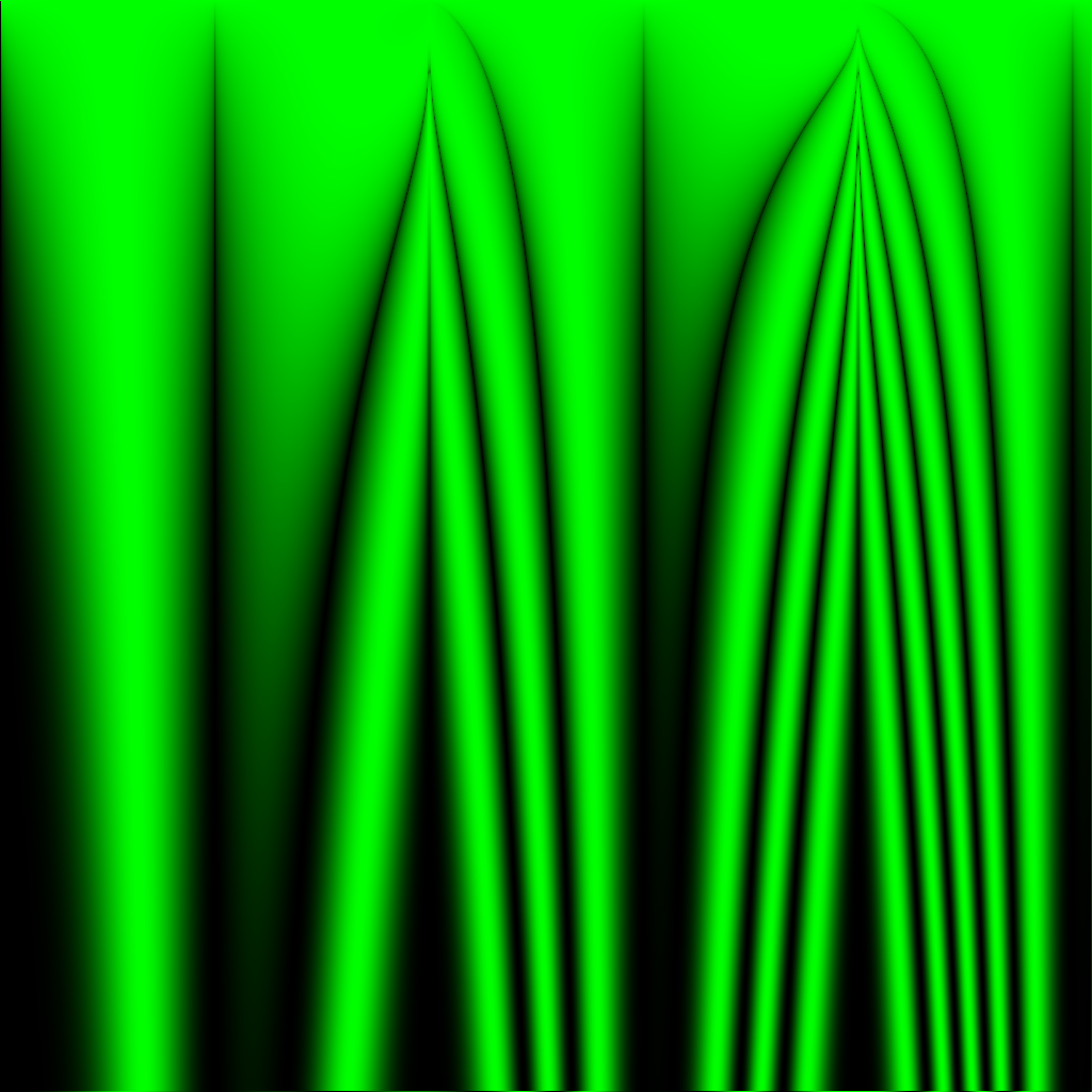
The result of Z -> abs(sin(sum(neighbors)*x/512))^(y/512) after 2 iterations.
In my recent simulations, I aim to search for ideal rules by testing all rules at once in a shared grid. Each cell’s position determines the parameters of the rule to be used, seen as the variables x and y in the image caption. Although no cell can interact with cells of the same rule, each cell will be interacting with cells of highly similar behavior, hopefully leading to large areas of an image all demonstrating good orderly behavior in areas centered around the pixel with the perfect parameters to create that behavior – just as the Mandelbrot set mimics whatever Julia set is formed by the value C equal to that location, but never perfectly re-creates a Julia set.
Y is measured from the top of the image in pixels, so in these 1024×1024 images, a rule definition which contains (y/512) means that that expression will range from 0 to 2 between the top edge of the image and the bottom edge.
In this entire post, I never resample images – each pixels corresponds to exactly one cell. Every cell state between 0.0 and 1.0 maps to a green channel value between 0 and 255 unless otherwise stated. Every simulation starts with all cells set to 0.5 unless otherwise stated.
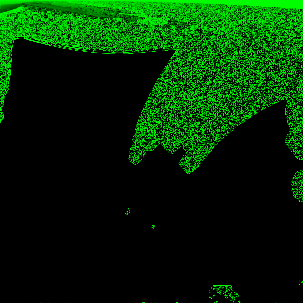
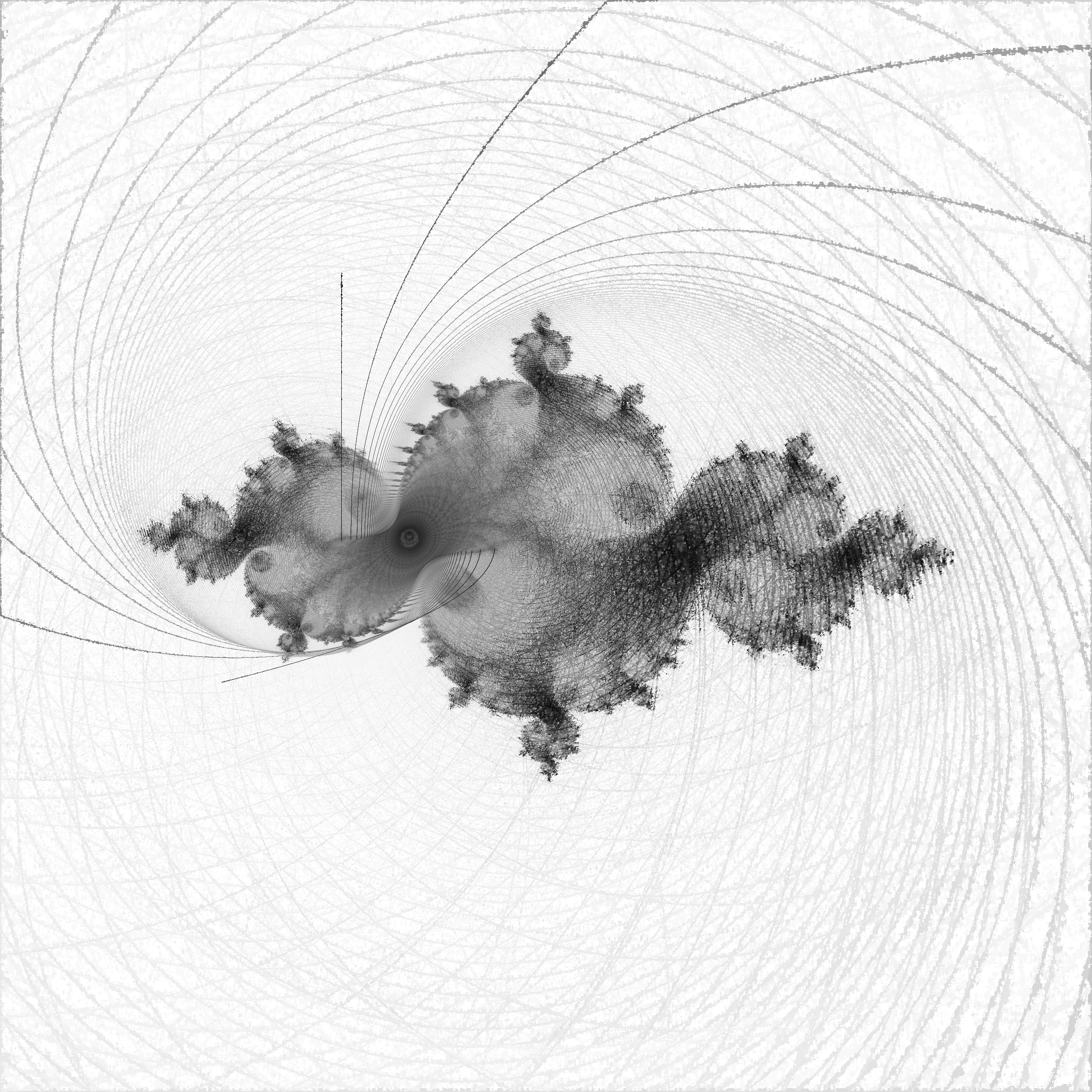
The result of Z -> abs(sin(sum(neighbors)*x/512))^(y/512) after 64 iterations.
The above image of the world at 64 iterations shows that, at least with the way I am choosing to initialize the world, there are no groups of similar rules that all create sparse activity. From images like these, I can’t determine what a only a few live cells would do in a vacuum, because none of them are alone without constant outside interference from other nearly-random cells… Starting with a few live cells is one of the best ways to demonstrate the strengths of Conway’s rule for creating complex organized motion, and this simulation doesn’t do that.
Good rules might be in there, and they just aren’t being given a fair chance at demonstrating order.
The result of Z -> abs(sin(sum(neighbors)*x/64))^(y/64) after 2 iterations.
This render is simply the first render zoomed out. Since there’s one cell per pixel, zooming out changes the number of cells in any area within the space of the parameters used for the rule, so zooming out must change the observed behavior of every part of the world. Cells that previously had neighbors with rule parameters different from their own by 1/512 now have neighbors with rule parameters different from their own by 1/64.
I zoomed out this far because I didn’t want to miss an interesting rule, but what I learned from zooming out this far was discouraging…
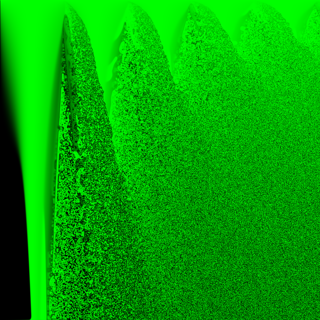
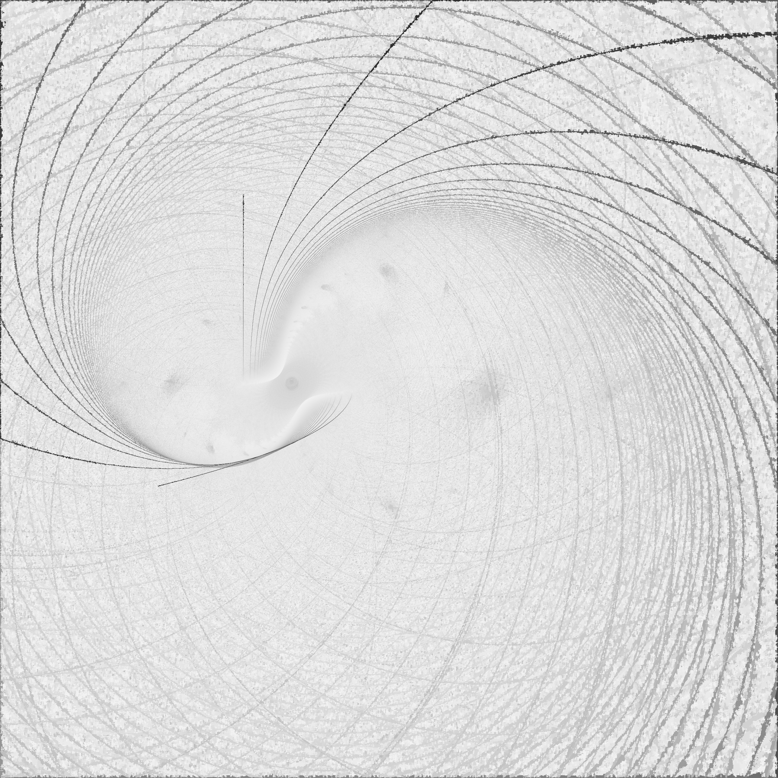
The result of Z -> abs(sin(sum(neighbors)*x/64))^(y/64) after 16 iterations.
The noise bleeds like ink until it fills up the whole world.
Generally, in Conway’s Game of Life, endless growth (of live cell population) is something that needs to be designed, not something that happens randomly. I can think of only one situation in which Conway’s Game of Life produces unlimited chaos…
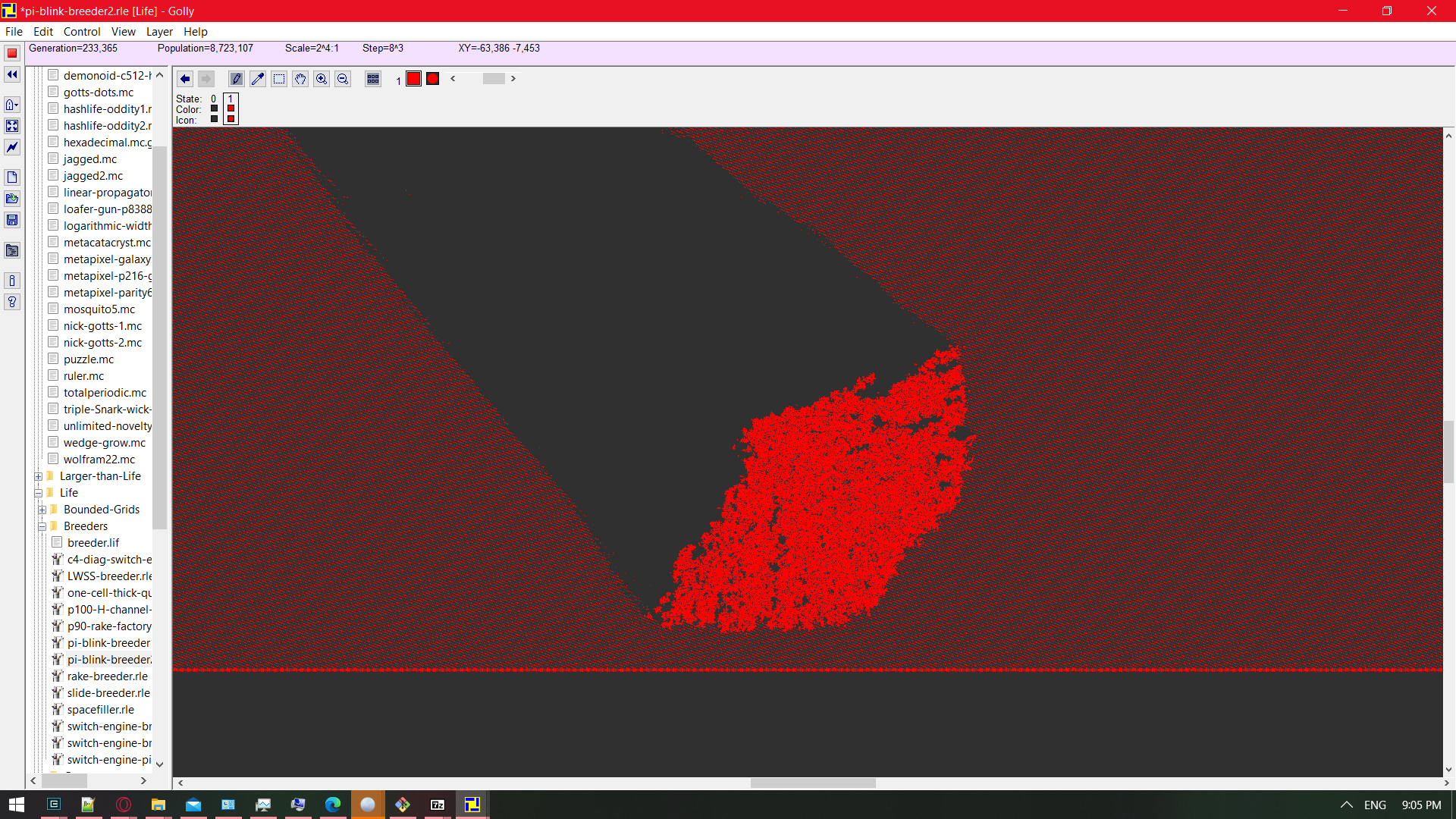
In an experiment I did in Golly, I required an infinite world of repeating gliders, and I used the preset pi-blink-breeder2 under patterns>Life>breeders.
pi-blink-breeder2
The pattern info includes this attribution:
#C An unusual breeder (quadratic growth) pattern.
#C By Jason Summers and David Bell, 6 Sep 2002; from "jslife" archive.
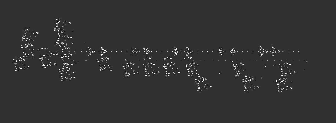
The breeder (a machine that constructs machines that construct gliders) is not important to the experiment – I am only concerned with the area of gliders it produces. In their midst, I drew exactly one glider traveling in the opposite direction, so that it collided with one of them after a while, and this was the result:
A noisy region of the world in Conway’s Game of Life, growing quadratically.
That’s essentially a ~200,000-car pileup, which would continue to grow infinitely if it didn’t hit the breeder’s wick of glider builders. In the best-behaved rule that I know of, all it takes to get an infinite chaotic mess is for the world to be initially full (of gliders).
If all I could see of this simulation were a section of the chaos coral, and I were asked whether I thought the rule that created it were Turing-complete, I might say “not really, I mean, you couldn’t practically make a computer out of it like you can with Life” not knowing that I was looking at Life.
I’m saying that none of my experiments so far offer strong evidence that a life-like rule using a sine function either does or doesn’t exist. In future experiments, I should test sine-based rules the same way I test rules by hand in Golly – apply the same rule to the whole world, edit in a handful neighboring live cells in a small random shape that isn’t symmetrical, and hit the play button. In FloatAutomata.py, this would look like quantizing the parameters of rules to make areas of about 64×64 cells that all have exactly the same rule, and not starting the simulation with every cell equal to 0.5. Each square of one rule should start with only a handful of nonzero cells in a cluster near the center.
In the meantime, here are the other experiments I’ve already performed with the whole world starting as 0.5-filled:
The result of Z -> abs(sin(sum(neighbors)*x/512))^(y/64) after 2 iterations.
The result of Z -> abs(sin(sum(neighbors)*x/512))^(y/64) after 16 iterations.
The result of Z -> abs(sin(sum(neighbors)*x/512))^(y/64) after 128 iterations.
It might seem like the boundary areas between emptiness and noise are good candidates for well-behaved rules, but I think that if this were true, the boundary areas would not constantly be moving!
Also note that toroidal wrap was enabled for every one of these experiments, and its effects can sometimes be seen in noise leaking in from the edges of an image to a maximum distance in pixels equal to the number of iterations to happen so far – it’s just because they were exposed to pixels on the opposite edge of the image. It usually doesn’t impact the image at the top or left edges, where one of the parameters is usually zeroed out anyway. For example, in the above image of Z -> abs(sin(sum(neighbors)*x/512))^(y/64) after 16 iterations, the bottom edge of the image has a line of noise caused by exposure to the top edge, but the top edge has no such line of noise.
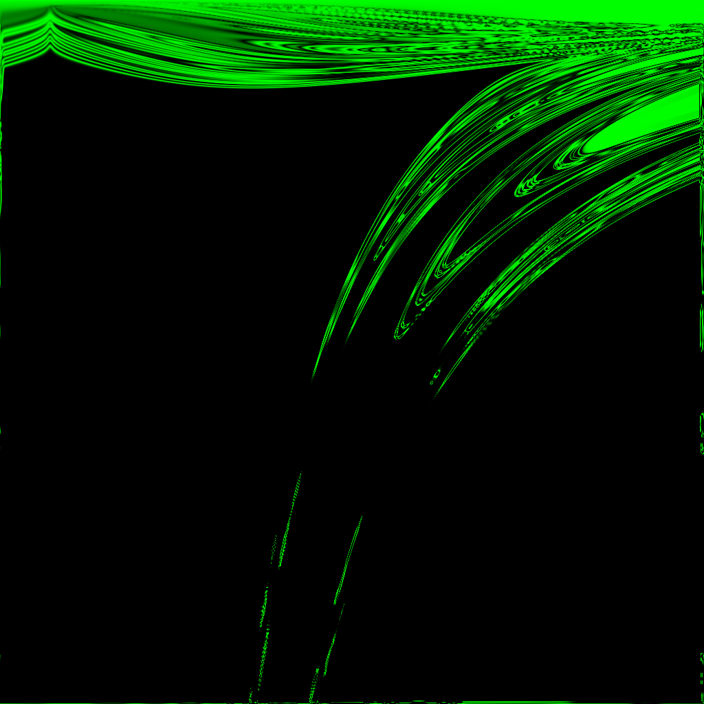
The result of Z -> abs(sin(sum(neighbors)*(0.375+0.25*x/1024)))^(y/64) after 1 iteration.
The result of Z -> abs(sin(sum(neighbors)*(0.375+0.25*x/1024)))^(y/64) after 2 iterations.
The result of Z -> abs(sin(sum(neighbors)*(0.375+0.25*x/1024)))^(y/64) after 8 iterations.
The result of Z -> abs(sin(sum(neighbors)*(0.375+0.25*x/1024)))^(y/64) after 64 iterations.
In the above images, anything that looks noisy is located very close to an area that was active in previous iterations – there are no gliders, and all things that look like islands of stability seem to eventually die. Except for two! their coordinates are (429, 720) and (518, 762), giving them the approximate rules:
Z -> abs(sin(sum(neighbors)*0.479736328125))^(11.25)
Z -> abs(sin(sum(neighbors)*0.50146484375))^(11.90625)
These will be investigated at a later date.
Even so, the above images serve to demonstrate that which areas of the image appear vital and stable is highly dependent on which areas of the image had ideal starting conditions from the few iterations after the world’s creation, which in turn depends on which rules are good at creating chaos from a starting neighborhood of 8 cells all with the state 0.5.
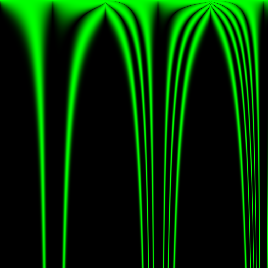
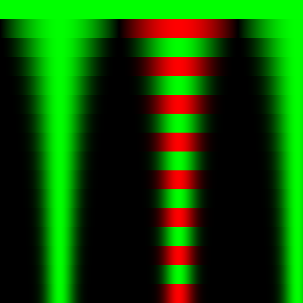
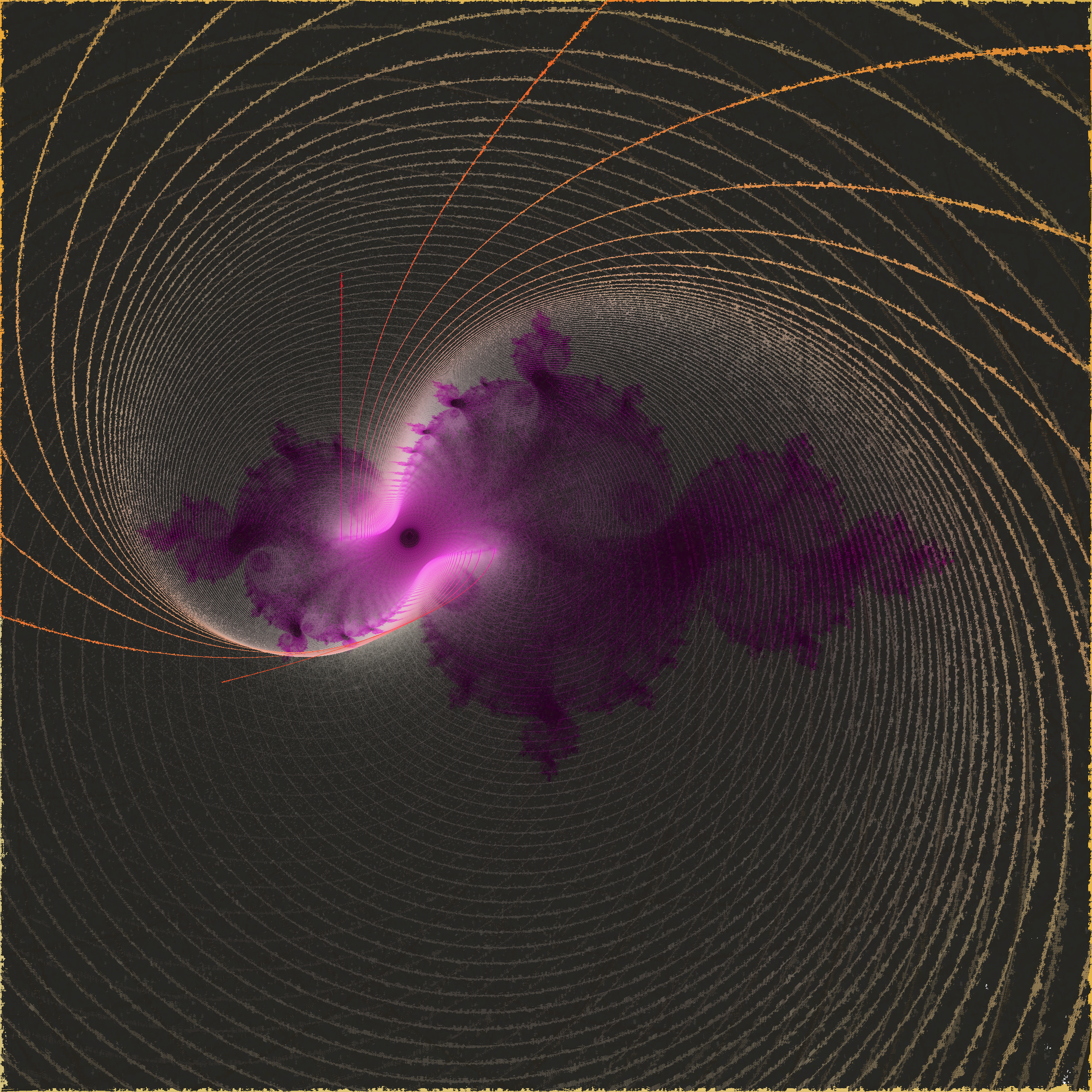
The result of Z -> sin(sum(neighbors)*x/512)^floor(y/64) after 1 iteration.
A new color palette has been introduced – reds code for negative values in the same range as greens. Negative numbers are allowed now that exponents are limited to integers – I didn’t want to deal with complex math on my first day of experimenting.
The result of Z -> sin(sum(neighbors)*x/512)^floor(y/64) after 4 iterations.
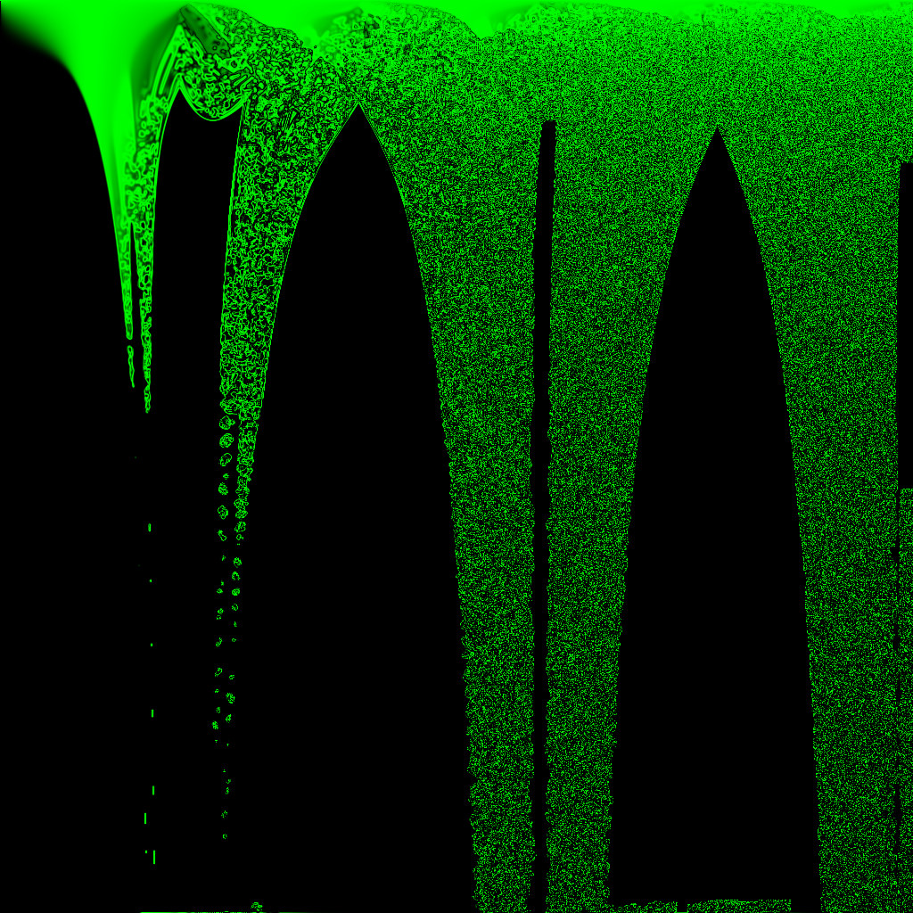
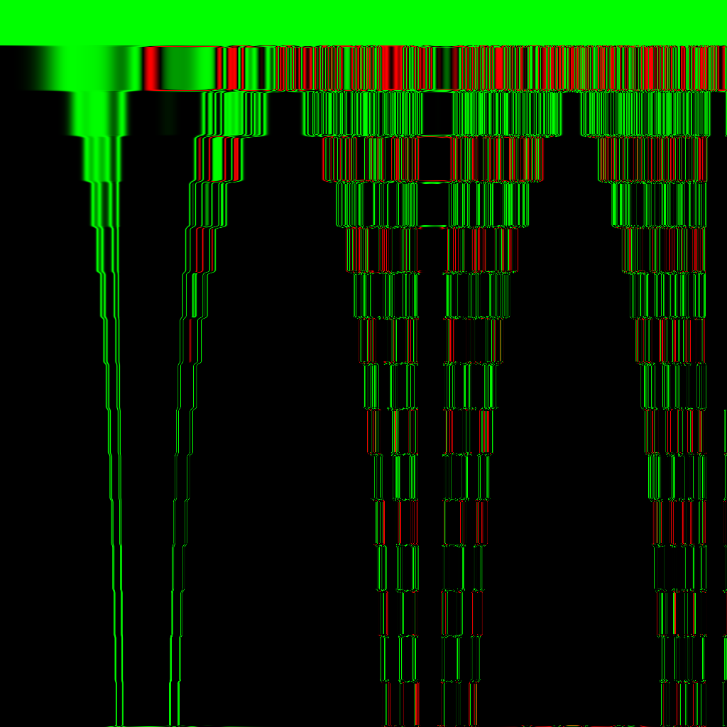
The result of Z -> sin(sum(neighbors)*x/512)^floor(y/64) after 24 iterations.
Note in the center left of the image, near the bottom end of the second of the image’s four tornado shapes, there appears to be a symmetrical barcode shape – animated over time, this looks like traveling along a binary tree layer by layer. Conway’s Game of Life never does this, but I believe some other cellular automata with binary states do. Just like what is seen here, those rules produce growing regions of noise at either end of a barcode’s bars until the barcode is consumed by the noise. In this experiment, the barcodes are initially stretched between the boundary lines of integer exponents in the rule (64 pixels per integer value).
I may upload additional experiments of the same type before continuing to testing of individual rules with more fair (non-solid) starting states of the world. I will also cover some surprisingly orderly rules using the tangent function!
The entire project is available on GitHub to view and download. It requires only Python to run. If you also have Pygame installed, it is used to draw graphs that supplement the console output.
For my semester project in 2017, I decided to finalize a program I had already been working on for several months as a hobby: An algorithm to travel between any two input numbers, using only the operations from the Collatz Conjecture to construct a path.
My goals for this project:
Demonstrate that a transformation between any two positive integers can be created by applying 4 unique operations in a finite sequence,
Compute the shortest sequence for two input numbers,
Provide an example of how these sequences can be used in cryptography.
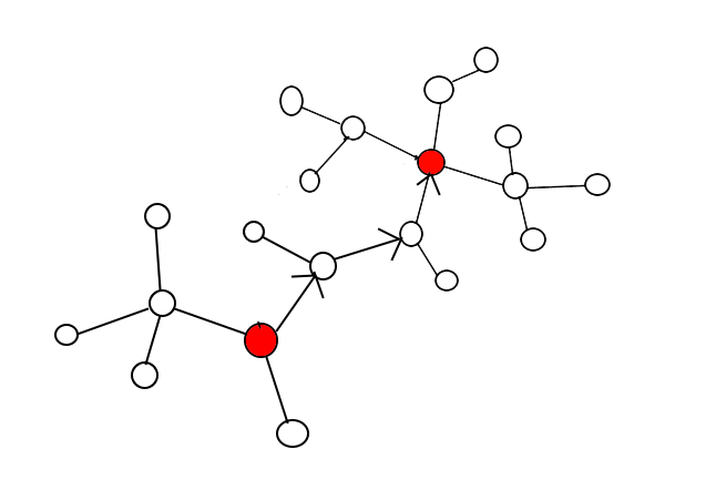
In the Collatz conjecture, the appropriate operation is chosen based on whether N is even or odd; N->N/2 is applied only when N is even, N->3N+1 is used otherwise. This ensures that N remains an integer, but also allows only one sequence of operations to occur after the starting point N. In my program, the inverses of these two operations (N->2N, N->(N-1)/3) are also available, and an operation is allowed whenever the result is an integer.
This gives freedom of movement throughout the number line.
Rather than selecting new operations based on a rule regarding the current number, a sequence can be created by an outside program, which has memory (See: the difference between Langton’s Ant and Langton himself). The numbers visited are like intersections in a maze, and the sequence generator acts like a maze solver.
I did not know about graph theory when I created this, but I ended up creating a breadth-first undirected graph search. The graph consists of all numbers which satisfy the Collatz conjecture, and the edges are the 4 operations.
The first version of the program was not so advanced – it searched by iteratively choosing the option which was closest to the target number, but avoiding numbers which had already been used. This was inefficient, and not set up to find the shortest path.
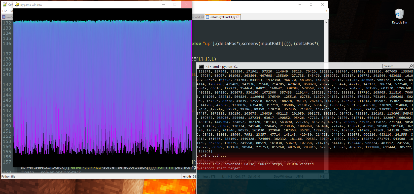
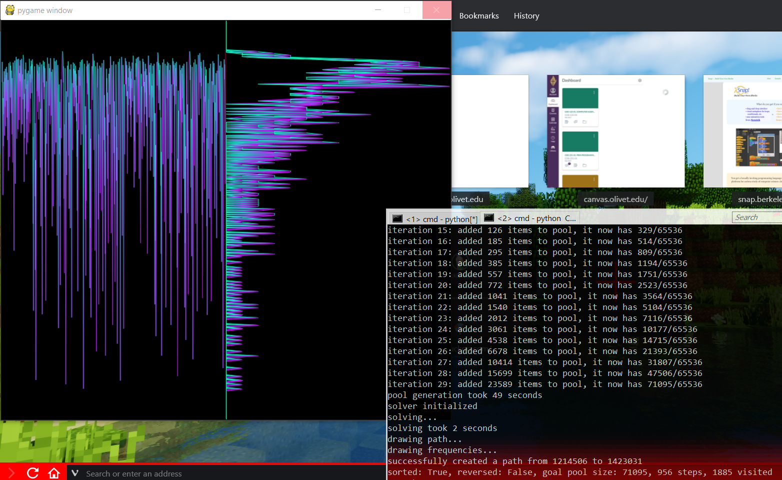
A particularly long path (166377 steps) found by the stacked solver. Horizontal axis is the index of the step taken, Vertical axis is the linear value of the number visited by a step. Values start at 0 at the top of the window and increase with distance
The quickest path to the target number would never be guessed by this solver, if any of the steps in the quickest path were not the longest steps that could be taken. That is to say, when creating a path from 64 to 256: 64 (*2) -> 128 (*2) -> 256
would always be turned down in favor of: 64 (*3+1) -> 193 -> (a lot of aimless wandering) -> 256
Originally, the stacked solver could become barred from reaching the goal by a wall of numbers that it had already used, and would be forced to walk further and further from the goal until it ran out of memory. (Even with edge prioritization, it turns out depth-first searches of infinitely large graphs often run out of memory. weird.)
I took 3 approaches to improving the performance (and reliability) of this method:
1. Sorting the history of visited numbers and using a sorted search.
2. Putting a limit on the highest value that can be visited, backtracking to find paths which stay below it.
3. Starting at the goal, Generate a pool of related numbers. terminate the depth-first search when it reaches any number in this pool.
I found that the third approach was very effective. Although preparing a large pool naturally required more memory, it required a predictable amount of memory, and consistently reduced the runtime of the stacked solver.
A depth-first search which ends upon reaching a value in a pre-generated goal pool
A much shorter path is found by creating a large goal pool, and allowing the Stacked Solver to run until it reaches a number present in the pool. The new graph on the right side of the window is a frequency map of how often different value ranges are visited by the solver; the vertical axes of the two graphs correspond directly.
In some experiments, it even reduced the runtime of the stacked solver to 0 steps: When the goal pool grows so large that it includes the starting value, the stacked solver doesn’t need to take any steps towards the goal. It is finished as soon as it starts. This led me to create my current version of the program, which doesn’t use a stacked solver at all – paths are found by creating two pools, one at the starting number and one at the goal, and expanding them both until they intersect.
Finding a shorter path by expanding two pools until they intersect, eliminating the Stacked Solver altogether
This method ensures that the first path found is the shortest possible, or shares this shortest possible length with other paths.
But the memory usage of these pools grows exponentially with the length of the shortest path.
In my next post, I will show how pools can be created with much lower memory usage, while maintaining or increasing performance. I’ll also cover the structure of the pools I used, how I navigated them to determine the path by which the intersecting items were generated, and how a program for graph navigation such as CollatzCrypt can be used to encrypt small payloads using a private key.
My semester project in Computer Science Principles was to create a program in Berkeley’s “Snap!” programming language, which we had learned to use in this semester. It needed to be more complex than our previous projects, and also have some social significance.
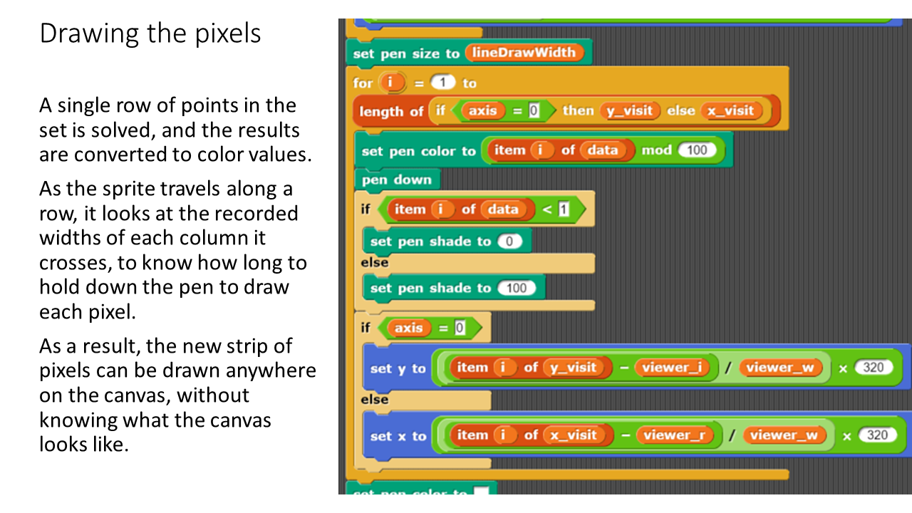
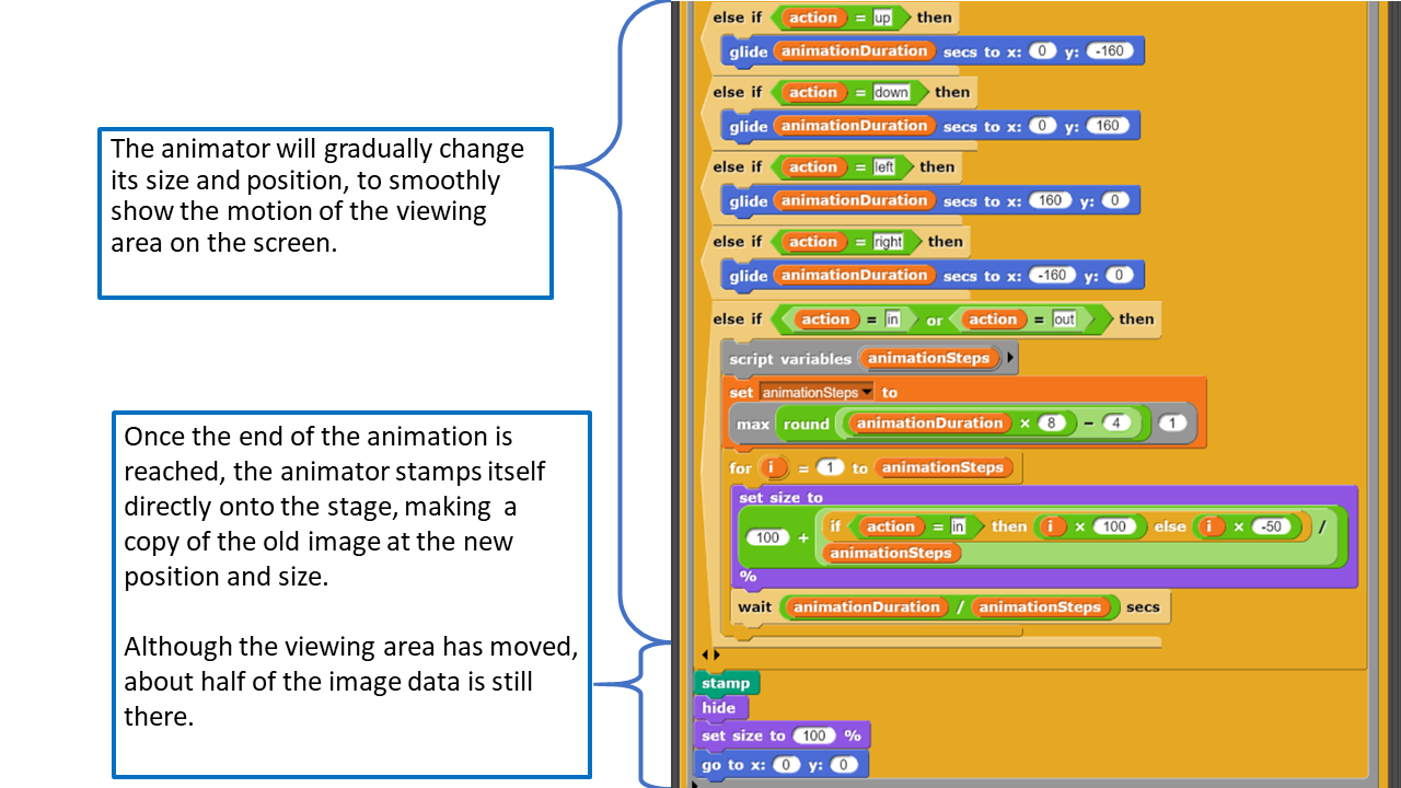
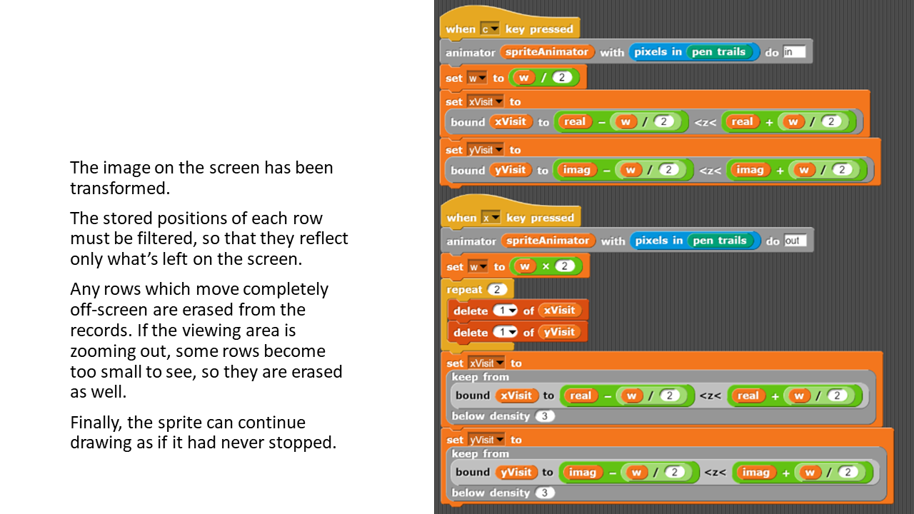
I decided to create a simplified and readable demonstration of the XaoS algorithm.
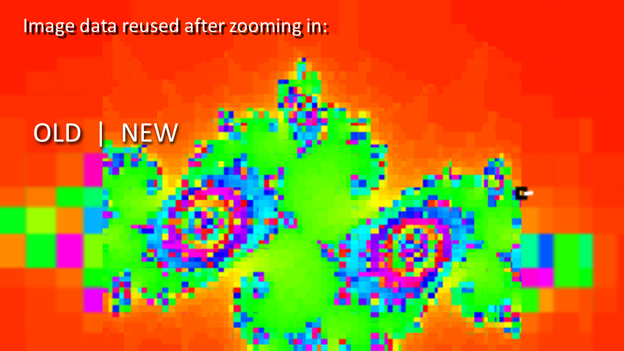
GNU XaoS is perhaps the fastest open source iterative fractal generator in the world. It inserts new rows and columns of pixels to refine the image without repeating any old calculations. My program demonstrates how this can be accomplished in a simple way.
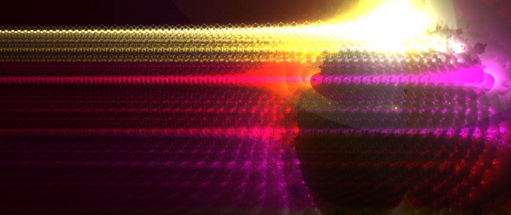
After I turned in Underground Lake as my final project, I wasn’t finished. So I kept working. I made this loop.
The background I made from a checkerboard, which I distorted+animated with Turbulent Displace and highlighted with Vegas. I pixelated it with the Mosaic effect to add sharp transitions, and then used a very complex Turbulent Displace to obscure the pixelation.
The Aurora effect was created with scatter, glow, and blur, applied to two overlaid audio spectrums. The blue had a short durational average of 45 milliseconds to respond to the beat, while the green spectrum averages over 360 milliseconds to reflect chords.
Saturday, I felt like learning how to use sockets. So I started to work on my first multiplayer game.
It’s nicknamed “flat” for now. It will get a real name when I know what the objective will be. Right now, you move around and invert the color of the gameboard wherever you go, watching others do the same (I planned on making this feature into a snake game).
The only thing significant about these random squares is that they were streamed from a separate process using python sockets.
After testing each new feature of python, I added code in large chunks, and managed to make the server multithreaded by Sunday. It now supports multiple connections.
Two clients connected to the same server.
The most important feature of this project is a single class I designed to handle data synchronization. The DataHandler class:
class DataHandler:
  def __init__(self,objects,name="unnDH"):
    self.objects = objects
    self.changes = {}
    self.name = name

  def __setitem__(self,key,value): #change something
    if not (self.changes.__contains__(key) and self.changes[key]==value):
      self.changes[key] = value

  def __getitem__(self,key): #shows unapplied changes
    return self.changes[key] if self.changes.__contains__(key) else self.objects[key]

  #removes all changes that don't contain a value that's actually new
  def cleanChanges(self):
    for key in self.changes:
      if self.objects.__contains__(key) and self.objects[key] == self.changes[key]:
        self.changes.delitem(key)

  #apply changes and empty changes dictionary
  def applyChanges(self):
    for key in self.changes:
      self.objects[key] = self.changes[key]
    self.changes = {}

  #encodes changes, also applies them locally
  def getUpdate(self):
    self.cleanChanges()
    result = str(self.changes).replace(" ","").encode()
    self.applyChanges()
    return result

  #encodes all data without emulating or applying changes
  def getRefresh(self):
    result = str(self.objects).replace(" ","").encode()
    return result

  def putUpdate(self,stream): #recieving data
    if type(stream)==DataHandler:
      updates = stream
    elif type(stream)==bytes:
      updates = eval(stream.decode())
    else:
      print(self.name + " putUpdate: unknown update type " + str(type(stream)) + " " + str(stream))
    for key in updates:
      #assume that if the held object is a DataHandler, its update must be a dataHandler update dictionary.
      if type(self.objects[key])==DataHandler:
        #updates are recursive, to change only parts of parts
        self.objects[key].putUpdate(updates[key])
      else:
        self.objects[key] = updates[key] #put regular update
    if len(self.changes) > 0:
      print(self.name + "flatData was given update while tracking changes. (bad things may happen now)")
This class allows the Server to properly handle game data during a game tick.
When the Server applies rules other mechanics to its data in a DataHandler, it sees the effects in real time – to the Server, the DataHandler is no different than a python dictionary object. Whenever a new client joins, the Server uses getRefresh() to send a complete copy of the data as it currently appears to all players, so that the new client is on the same page as everyone else.
However, when the game tick is over, the server uses getUpdate() to send each client a copy of only the data that has been changed in this game tick. Calling getUpdate() applies all of the changes to the core data and empties the change list, and the DataHandler is ready for the next tick to begin.
DataHandlers are good for complex data, because they encode and evaluate strings without complicated conversions specific to the type of data (any primitive can be sent without writing new code). They can even be nested, to recursively send only parts of parts, and so on. That’s my most important accomplishment so far.
However, none of these optimizations are currently applied to the board, which is hundreds of times larger than the player data updates. I will need to create a separate class of data handler for tracking array changes.
Next on my list of priorities:
Create an array data handler.
Round out the access methods of DataHandler to where it can be used recursively, tracking and emulating changes from as many ticks as there are levels of linked DataHandlers. Updates will be given to clients according to how long they have been unresponsive, unless they have been unresponsive for longer than changes are tracked.
Refactor Server to have a self-contained game controller that isn’t responsible for networking.
Run game controller outputs through a filter to remove data that’s irrelevant to the player (off-screen movement, etc.)
Scan for servers (right now the code only checks for servers running on this computer.)
Redesign DataHandlers to remove the hard-coded distinctions between server access and client access. Instead support the creation of viewer identities, through which data is accessed – automatically tracking which clients have received or sent which data, but without duplicating any data internally.
2 days ago, I imagined the programming styles that would be possible with a ‘can’ statement, which allows methods of a class to be declared outside of a class at any time during execution. My goal was to allow programs to be written in the order that you have new ideas, or in the order that they are explained in a summarized writing.
I outlined two python projects of identical function: a normally structured project and a can-statement project. The function of each project was to simulate and show Langton’s Ant.
original version:
#there is a Board class
# a Board can prepare(ruleset) its Ants' AI
# a Board can advance() its Ants
# a board can inform & control its Ants with step()
# a Board can display() itself
#there is an Ant class
# an Ant can move()
# an Ant can turn()
# an Ant can bound()
#there is an AI class
# an AI can decide(condition) how to turn
# an AI can influence(condition) the current square
#create a Board called "world"
#tell world to prepare(ruleset)
#loop:
# tell world to advance()
# tell world to display()
‘can’ statement version:
#there is a Board class.
#there is an Ant class.
#an Ant can move()
#an Ant can turn()
#there is an AI class.
#an AI can decide(condition) ho to turn
#an AI can influence(condition) the current square
#Boards can prepare(ruleset) their Ants' AI
#an Ant which is the child of a Board can step()
#an Ant which is the child of a Board can bound()
#a Board can advance() its Ants
#a Board can display() itself
#create a Board called "world"
#tell world to prepare(ruleset) its Ants.
#loop:
# tell world to advance()
# tell world to display()
It might be good for drafts, but it isn’t helping if it causes you to delay memorization of the structure of the project. It also becomes messier and harder to jump into. Perhaps it can be used to write first drafts of classes, and then converted to regular python before classes get very large.
In combination with ‘can’ statements, the example uses ‘of’ statements, which allow methods to be created in the context of both an object and its parent.
Ant of Board can Bound(self,parent):
  self.x %= parent.width
  self.y %= parent.height
I took both outlines and created real python projects out of them. The ‘can’ statement version isn’t runnable, but for a while, I updated it to fix errors I found in the working version. It would work if I could compile it. I’ll clean up both projects and publish them soon.
My program’s output after running the first 11208 iterations of the basic LR Langton’s ant. The board wraps around, so the Ant isn’t able to build an infinite highway.
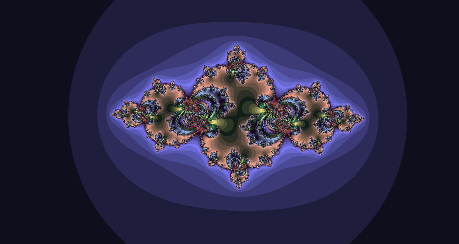
In my earlier experiments, I placed the starting points of a Buddhabrot generator along a line through the Mandelbrot set. The points starting below the real axis produced a mirror image of those that started above, and a lot of detail was wiped out when the two images were blended. From now on, any vertical lines will be cut off at the real axis, and the asymmetry will be visible.
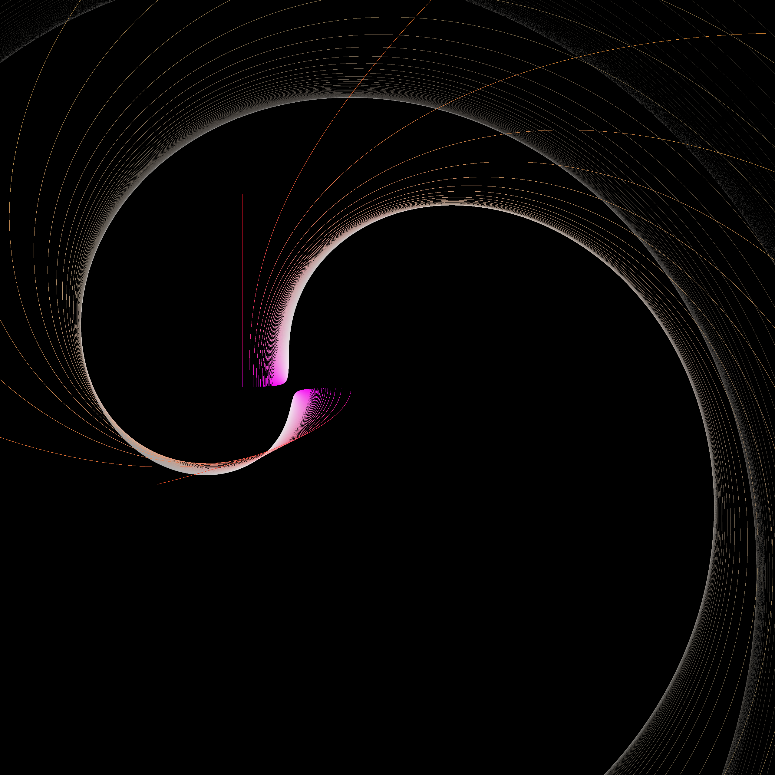
Here’s the non-mirrored Buddhabrot of seahorse valley:
When moved slightly to the right, the line of starting points begins to cut into the seahorses and into the cardioid itself. The Buddhabrot then forms the image of a seahorse Julia set.
Starting points lined up at -0.75+1/4096 (-0.749 755 859 375)
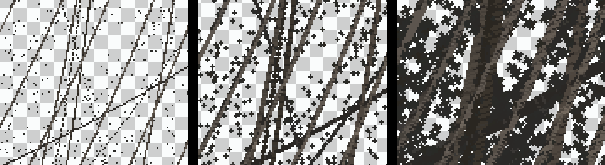
Most pixels in the image are pure black, so I wanted to interpolate all color data from the non-black pixels before starting to refine the image.
I will eventually automate this, because I know I’ll want to do it again. But for now, I’m working with Photoshop. I deleted all black pixels, and tessellated the remaining pixels to fill the gaps. I did this by duplicating the layer 5 times, arranging the duplicates into a tiny pinwheel, merging them, and repeating.
First 2 steps of manual tessellation
The result after 5 steps
When the green channel is divided by the red channel, it yields the original measurements of progression of a point.
Luminosity = progress towards escaping
Perhaps the most interesting thing about this fractal is that it isn’t simply composed of points that started very near the real axis. The blue channel divided by red is not very distinct:
Luminosity = closeness of starting point to the real axis
I’ll continue to work on explaining exactly how this type of fractal can be found, and also, how different it is from the basic seahorse Julia set.
C=-0.75+0.05i: Seahorse valley Julia set, generated with XaoS.
For my final project in interactive media, I composed “Underground Lake” with LMMS. Then, I challenged myself to visualize the music as a pattern of moving ripples in a dark pool of water.
The purpose of this project was to overcome a barrier in After Effects, the lack of a feature that seems fairly simple: A way to transform the composited image data in the Echo effect. For instance, creating a trail for a stationary object.
It would be so simple, if only you could:
reference the image of this layer “current” as it appeared 1 frame ago, through the virtual layer “last”
apply the transform effect to “last”
composite “last” on top of “current”
The Echo effect is sealed shut, and doesn’t allow that kind of tinkering. This project is a hack, using MotionTile to animate layer trails.
My final submission also included a diagram of the entire project. However, I think that my diagram could be refined before I post it here. In the meantime, here’s the video:
I read somewhere recently – as you approach the real axis of the Mandelbrot set near -0.75 (seahorse valley), the number of iterations before a point escapes, multiplied by the distance to the axis, approaches pi.
It’s a cool fact about the Mandelbrot set. but it isn’t a practical way to calculate pi; it takes a 2*10^n calculations to calculate n digits.
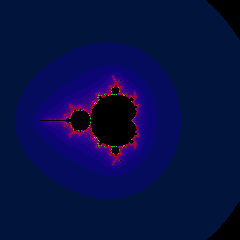
I wanted to know what points in the Mandelbrot set actually did in this area. So I rendered a Buddhabrot with starting points placed along a vertical slice at -0.75:
This is zoomed out a ways. Here’s the Mandelbrot set at the same zoom level for reference:
Each line represents a common iteration level for the points of the starting line. each line is completely continuous, because the input function is continuous and the iterated function is too.
As soon as I saw this, I decided to do vertical slices of the entire set.
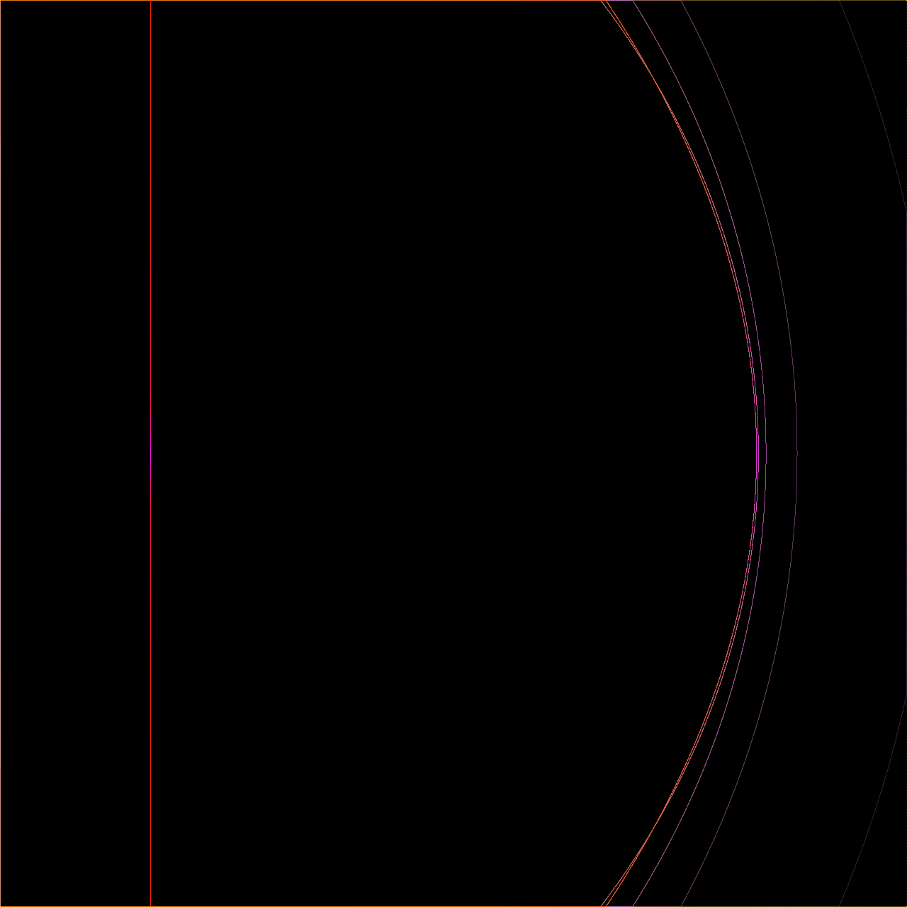
In the following images,
The blue channel indicates how close to the real axis a point started. The bluer it appears, the smaller the imaginary component of c is.
The green channel indicates how far a point has moved through it’s lifetime. If a point takes 500 iterations to escape, it will be drawn with 80% green channel brightness on its 400th iteration.
The red channel is the reference for the others – it is simply brighter when a pixel is visited more often, and represents the highest value any of the other channels could be for that pixel. (At rasterization time, other channels are multiplied by red and divided by 255.)
slice 213/1280 (near the end of the spire)
slice 336/1280 (through the spire, near a mini-Mandelbrot which is causing the lines to curl)
slice 476/1280 (through the period 2 bulb, just to the left of seahorse valley)
slice 485/1280 (through the cardioid, just to the right of seahorse valley)
This sequence could be turned into an animation, but it’s quite large for a gif, So I’m looking to post it in a video. I also have several other discoveries to write about soon.